
Section 2.5 Continuity
Motivating example:
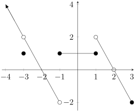
Loosely: A function is continuous if it is unbroken; it can be drawn without lifting the pencil. In the graph above, there are discontinuities at \(x=-3\text{,}\) \(x=-1\text{,}\) \(x=1\text{,}\) and \(x=2\text{.}\)
Definition 2.5.2. Continuous at a point.
Let \(f\) be a function and \(c\) a real number.
The function \(f\) is continuous at \(c\) if \(\displaystyle\lim_{x\rightarrow c} f(x)=f(c)\text{.}\) Note that this encompasses three conditions: that \(f\) is defined at \(c\text{,}\) that the limit exists at \(c\text{,}\) and finally that the limit at \(c\) equals the value of the function at \(c\text{.}\)
The function \(f\) is left-continuous or continuous from the left at \(c\) if \(\displaystyle\lim_{x\rightarrow c^-} f(x)=f(c)\text{.}\)
The function \(f\) is right-continuous or continuous from the right at \(c\) if \(\displaystyle\lim_{x\rightarrow c^+} f(x)=f(c)\text{.}\)
Remark 2.5.3.
We say that a function is continuous at a point \(x=c\) when \(c\) is a boundary point of its domain and it is left- or right-continuous there, in addition to when \(c\) is an interior point and it is continuous at \(c\text{.}\)
The function graphed above is continuous at \(x=-2\) since \(\displaystyle\lim_{x\rightarrow -2} f(x) = 0 = f(-2)\text{.}\)
It is continuous from the left at \(3\) since \(\displaystyle\lim_{x\rightarrow 3^-} f(x) = -2 = f(3)\text{.}\)
Definition 2.5.4. Continuous on a closed interval.
A function \(f\) is continuous over a closed interval \([a,b]\) if it is:
Continuous from the right at \(x=a\)
Continuous from the left at \(x=b\text{,}\) and
Continuous at every interior point, that is, at every point in \((a,b)\text{.}\)
We define continuity on the half-closed infinite intervals \([a,\infty)\) and \((-\infty,b]\) similarly by omitting the condition for the endpoint that is not used.
So the function above is continuous on \([-1,1]\text{;}\) it is also continuous on \((-\infty,-4]\) and on \((-3,-1)\text{.}\)
Definition 2.5.5. Some types of discontinuities.
We have seen several types of discontinuities:
A discontinuity at \(x=c\) is removable if \(\displaystyle\lim_{x\rightarrow c} f(x)\) exists but is not equal to \(f(c)\text{.}\)
A discontinuity at \(x=c\) is a jump discontinuity if the left and right limits both exist but are different.
A function has an infinite discontinuity at \(x=c\) if it is unbounded around \(c\) (e.g., \(f(x)=\frac{1}{x}\)).
A function has an oscillating discontinuity at \(x=c\) if it is bounded but fails to have a limit because it oscillates too rapidly near \(c\) (e.g., \(f(x)=\sin \frac{1}{x}\)).
Definition 2.5.6. Continuous function.
A function is called a continuous function if it is continuous at every point of its domain. If there are one or more points in the domain of the function at which is is continuous, then it is a discontinuous function.
The function \(f(x)=\frac{1}{x}\) is a continuous function, because it is continuous at every point of its domain. That's not inconsistent with saying that it is not continuous at \(x=0\text{.}\)
Fact 2.5.7.
If \(f\) and \(g\) are functions that are continuous at \(x=c\text{,}\) then algebraic combinations are continuous at \(x=c\text{:}\)
Sums: \(f+g\)
Differences: \(f-g\)
Constant multiples: \(kf\) for a number \(k\)
Products: \(fg\)
Quotients: \(\frac{f}{g}\text{,}\) provided \(g(c)\neq 0\)
Powers: \(f^n\text{,}\) for \(n\) a positive integer
Roots: \(\sqrt[n]{f}\text{,}\) provided the root is defined on an open interval around \(c\)
Example 2.5.8.
Determine the set of \(x\)-values where the function is continuous:
\(\displaystyle f(x) = \sqrt[4]{4x-5}\)
\(\displaystyle g(x) = \frac{x-3}{2x^2-5x-3}\)
\(\displaystyle h(x) = \begin{cases} \frac{x-3}{2x^2-5x-3}\amp x\neq 3\\ \frac{1}{7} \amp x=3 \end{cases}\)
\(\displaystyle \displaystyle\left[\frac{5}{4},\infty\right)\)
\(\displaystyle (-\infty,-1/2)\cup(-1/2,3)\cup(3,\infty)\)
\(\displaystyle (-\infty,-1/2)\cup(-1/2,\infty)\)
Fact 2.5.9.
If \(f\) is a continuous function, then \(f^{-1}\) is continuous.
Fact 2.5.10.
The composition of continuous functions is continuous. That is, if \(f\) is continous at \(c\) and \(g\) is continuous at \(f(c)\text{,}\) then \(g \circ f\) is continuous at \(c\text{.}\)
Fact 2.5.11.
If \(g\) is continuous at \(x=b\) and \(\displaystyle\lim_{x\rightarrow c} f(x) = b\text{,}\) then
Example 2.5.12.
Find the limit: \(\displaystyle \lim_{x\rightarrow 0^+} \sin\left( \frac{5\pi}{6} e^{\sqrt{x}}\right)\)
Is \(\displaystyle \sin\left( \frac{5\pi}{6} e^{\sqrt{x}}\right)\) continuous at 0?
\(\sin(\frac{5\pi}{6}) = \frac12\text{;}\) yes
Fact 2.5.13. Intermediate Value Theorem.
If \(f\) is continuous on the closed interval \([a,b]\) and \(y_0\) is any number between \(f(a)\) and \(f(b)\text{,}\) then there is a \(c\) in \([a,b]\) such that \(f(c)=y_0\text{.}\)
One consequence of the IVT is that it guarantees the existence of roots:
Example 2.5.14.
Let \(f(x) = x^5 - 3x^3 + 5x-2\text{.}\) Since polynomials are continuous and \(f(0)\lt 0\) and \(f(1)\gt 0\text{,}\) there must be a real root \(0\lt c\lt 1\) such that \(f(c)=0\text{.}\)