CalcNotes Exponential Functions

Section 1.5 Exponential Functions

Note: in the textbook, this section contains a lot of applied problems about the exponential model of growth. This comes up again in Calculus II, so if you're planning on taking that class, it would be worth your time reviewing those examples.

Definition 1.5.1. Exponential Function.

For a constant \(a\gt 0\) with \(a \neq 1\text{,}\) the function \(f(x)=a^x\) is the exponential function with base \(a\text{.}\)

Example 1.5.2. Bacterial Reproduction.

30 bacteria are placed in a Petri dish. Each bacteria divides once per hour. Let \(b(t)\) be the number of bacteria after \(t\) hours. Find a formula for \(b(t)\text{.}\)

Solution.

\begin{align} b(0) \amp = 30\tag{1.5.1}\\ b(1) \amp = 30 \cdot 2\tag{1.5.2}\\ b(2) \amp = 30 \cdot 2^2\tag{1.5.3} \end{align}

We see that \(b(t)=30 \cdot 2^t\text{.}\)

Example 1.5.3.

Suppose instead that the bacteria triple every 10 minutes. Find a formula for \(c(t)\text{,}\) the number of bacteria after \(t\) hours.

Solution.

\begin{align} c(0) \amp 30\tag{1.5.4}\\ c(10\text{ minutes}) \amp = 30 \cdot 3\tag{1.5.5}\\ c(20\text{ minutes}) \amp = 30 \cdot 3^2\tag{1.5.6}\\ c(30\text{ minutes}) \amp = 30 \cdot 3^3\tag{1.5.7}\\ c(1) = c(60\text{ minutes}) \amp = 30 \cdot 3^6\tag{1.5.8} \end{align}

We see that \(c(t)=30 \cdot 3^{6t}\text{.}\)

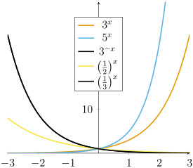
Example 1.5.4. Graphs of Exponential Functions.

Sketch graphs of the following exponential functions:

\(\displaystyle y=3^x\)
\(\displaystyle y=5^x\)
\(\displaystyle y=3^{-x}\)
\(\displaystyle y=\left(\frac{1}{2}\right)^x\)
\(\displaystyle y=\left(\frac{1}{3}\right)^x\)

Answer.

Graph of the functions in the example — Figure 1.5.5. Graph of some exponential functions

Fact 1.5.6. Rules for Exponents.

For positive real numbers \(a\) and \(b\text{:}\)

\(\displaystyle a^x a^y = a^{x+y}\)
\(\displaystyle (a^x)^y = a^{xy}\)
\(\displaystyle \frac{a^x}{a^y} = a^{x-y}\)
\(\displaystyle a^x b^x = (ab)^x\)
\(\displaystyle \frac{a^x}{b^x} = \left(\frac{a}{b}\right)^x\)

Definition 1.5.7. Natural Exponential.

The natural exponential function is the exponential function with base \(e\approx 2.718281828459\text{.}\) It can be written as \(e^x\) or \(\exp(x)\text{.}\)

Fact 1.5.8.

All basic exponential functions, i.e., \(f(x)=a^x\) have \(y\)-intercept \((0,1)\text{.}\) One of the features of the natural exponential is that its slope is 1 at \((0,1)\text{.}\)

Definition 1.5.9. Continuous Exponential Growth and Decay.

The equation \(y=y_0e^{kx}\) models exponential growth and decay, where:

\(y_0\) is the initial quantity, the amount at time 0; note that \((0,y_0)\) is the \(y\)-intercept.
\(k\) is the growth constant, controlling the rate of growth (for \(k\gt 0\)) or decay (for \(k \lt 0\)).

Example 1.5.10. Graphing exponential growth/decay.

Sketch graphs of:

\(\displaystyle y=3e^x\)
\(\displaystyle y=3e^{2x}\)
\(\displaystyle y=3e^{x/2}\)
\(\displaystyle y=3e^{-2x}\)
\(\displaystyle y=-3e^x\)

Answer.

Link to graphs in Desmos ¹

www.desmos.com/calculator/yosp3sjv0k